Safety Stock Calculator & Reorder Point

Safety Stock Calculator & Reorder Point

Calculate optimal safety stock, reorder point (ROP), and Z-score across variable lead time and demand. Prevent stockouts and optimize holding costs.

Lbl regime currency
Lbl presets
Lbl variability mode
Lbl service level95.0Symbol percent(Lbl z score prefix1.645)

Hint stockout prob

Lbl demand distribution
Lbl lead time parameters
Lbl economic factors
Lbl algorithmic complexity
Lbl policy active continuousLbl z score short 1.645
Hero safety stockHero safety stock badge
682Unit units

3.8 Unit days of supply Lbl coverage

Hero reorder pointHero rop badge
2,482Unit units

Lbl trigger order at

Hero annual holding costHero holding badge
$4,859.25Unit currency per year

$19,437.00 Lbl capital tied up short

Hero stockout riskHero risk badge
5.00Symbol percent

95.0Symbol percent Lbl guaranteed availability

Sec lead time demand1,800.0 Unit unitsD (180) × L (10)
Sec active z1.6449norm_inv(95.0%)
Sec buffer days supply3.8 Unit daysSS (682) / D (180)
Sec demand variance share24.6Symbol percent
Sec lead time variance share75.4Symbol percent
Sec working capital tied$19,437.00682 units × 28.5
Title formula breakdown
Formula step1
σ_LTD = √(10.0 × 65² + 180² × 2²) = 414.55 units
Formula step2
SS = Z (1.645) × σ_LTD (414.55) = ⌈681.87⌉ = 682 units
Formula step3
ROP = LTD (1800.0) + SS (682) = 2482 units
Lbl engineLbl bivariate model
Lbl zero server egressLbl last updated
Primary Metric95.0Symbol percent (5.0Symbol percent Lbl risk suffix)
Efficiency / Capacity$4,859.25 Unit currency per year
Net Output3.8 Unit days Lbl coverage

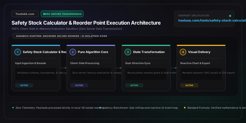
Client-Side Processing

High-performance calculation executed entirely in browser memory.

Zero Server Upload Privacy

All payloads remain strictly local with zero external server communication.

Production Ready Export

Clean, optimized output formats ready for immediate deployment.
Technical Reference & Architecture Guide

Safety Stock Calculator & Reorder Point Guide

Calculate optimal safety stock, reorder point (ROP), and Z-score across variable lead time and demand. Prevent stockouts and optimize holding costs.

Safety Stock Calculator & Reorder Point Guide — Client-Side In-Memory Architecture & Data Flow

Key Parameters & Controls

average_daily_demandUnits / Day (Mean Consumption Velocity)

Arithmetic mean daily consumption (D̄ = Σx_i / n) across an unconstrained 30 to 90-day demand window. Standard supply chain baselines require filtering out unfulfilled stockout periods to prevent artificial downward bias in baseline velocity.

Default: 100
demand_standard_deviationUnits (Demand Volatility σ_D)

Sample standard deviation of daily sales calculated via Bessel-corrected variance (n - 1 denominator). For fast-moving consumer goods (FMCG), a coefficient of variation (CV = σ_D / D̄) exceeding 0.50 denotes high volatility requiring intermittent Poisson or negative binomial modeling rather than standard Gaussian assumptions.

Default: 15
average_lead_time_daysDays (Supplier Replenishment Latency L̄)

Mean procurement latency spanning purchase order generation, vendor manufacturing, transit, customs clearance, and warehouse dock-to-stock putaway. For overseas container freight, benchmark latency spans 28–45 days; domestic distribution averages 3–7 days.

Default: 14
lead_time_standard_deviationDays (Procurement Transit Variance σ_L)

Standard deviation of supplier order fulfillment latency across historical replenishment batches. In King's bivariate formulation, lead time variance acts as a squared multiplier against average demand (D̄² × σ_L²), frequently contributing over 70% of total stockout exposure in global sourcing.

Default: 3
cycle_service_levelPercentage (CSL / Non-Stockout Probability [0.50, 0.999])

Target non-stockout probability during a single replenishment cycle, mapped to standard normal distribution quantile Z = Φ⁻¹(CSL). Standard e-commerce catalog baselines target 95.0% (Z = 1.645); high-margin or contractual SLA accounts target 98.0% (Z = 2.054) to 99.0% (Z = 2.326).

Default: 95.0%
annual_holding_cost_rateAnnual Percentage Rate (H / Carrying Cost [0.15, 0.35])

Total annualized capital and operational cost incurred to carry one unit of inventory, comprising Weighted Average Cost of Capital (WACC), warehouse real estate, insurance, shrinkage, and obsolescence. Standard industrial benchmarks range from 20% to 30% per annum.

Default: 25.0%

Pro Tips & Best Practices

Lead Time Variance Trumps Demand Volatility via King's Quadratic Term

In bivariate environments, safety stock is governed by King's equation: SS = Z × √[L̄ × (σ_D)² + D̄² × (σ_L)²]. Because lead time standard deviation (σ_L) is multiplied by average demand squared (D̄²), a slight supplier delivery jitter of 2 days on a 200 unit/day SKU introduces 160,000 units of variance to the radicand, dwarfing daily sales volatility. Prioritize vendor lead-time consistency SLAs over demand forecasting refinement.

Correct for Periodic Review Cycles Using (L + R) Protection Windows

Standard Reorder Point (ROP = D̄ × L̄ + SS) assumes continuous review where inventory position is evaluated in real time via automated WMS triggers. If purchase orders are batched periodically (e.g., weekly review period R = 7 days), the vulnerability window extends to L + R. Calculate safety stock over √[L + R] rather than √L; failing to expand the exposure interval systematically guarantees an actual service level 10–15% below target.

Client-Side O(n) Single-Pass Variance Prevents Enterprise Data Exfiltration

Processing proprietary 365-day enterprise sales histories client-side in the browser execution sandbox via Welford's numerically stable O(n) recurrence algorithm (M_k = M_{k-1} + (x_k - M_{k-1})/k) maintains absolute data confidentiality. By avoiding server-side POST requests, proprietary ERP SKU demand patterns and unit margins remain isolated within local memory, eliminating supply-chain reconnaissance attack surfaces.

Guard Against Gaussian Breakdown on Intermittent or Fat-Tailed SKUs

The standard normal Z-factor assumes independent and identically distributed (i.i.d.) Gaussian demand. When calculating safety stock for intermittent 'lumpy' demand (Croston's pattern where CV > 0.75 or zero-demand days exceed 30%), the Gaussian assumption underestimates safety buffer requirements by 20–40% at high service levels (≥98%). Substitute parametric models with Bootstrapping or Negative Binomial distributions for slow-moving tail SKUs.

Common Gotchas & Troubleshooting

⚠️Calculated Reorder Point Yields Fractional Units or Negative Lead Time Demands

Always apply ceiling integer quantization (Math.ceil(ROP)) rather than standard rounding to prevent sub-unit stockout vulnerability during discrete picking operations. If ROP evaluates to negative values, verify that raw demand inputs represent positive consumption; negative returns or credit memos in ERP transaction feeds must be isolated from gross sales velocity.

⚠️Acklam's Inverse Normal CDF Approximation Diverges at Extreme Service Levels (>99.9%)

For service levels approaching 1.0 (e.g., aerospace spares at 99.99%), rational Chebyshev polynomial approximations for Φ⁻¹(p) experience IEEE 754 double-precision floating-point catastrophic cancellation. Constrain input bounds strictly within 50.0% ≤ CSL ≤ 99.95% (Z ≤ 3.29), or switch to high-precision asymptotic series expansions for extreme tail quantiles.

⚠️Unadjusted Stockout Periods Artificially Depress Sample Mean and Volatility

When inventory hits zero, recorded sales drop to zero regardless of true market demand. Ingesting unadjusted zero-sales days compresses both D̄ and σ_D, inducing a systemic downward spiral in calculated safety stock (the 'phantom inventory trap'). Pre-process time-series data to censor out-of-stock timestamps or impute latent demand via historical run-rates before running the King variance estimator.

Frequently Asked Questions

How do you calculate safety stock with variable lead time and demand?▼

Use King's bivariate inventory formula: Safety Stock = Z × √[L × (σ_D)² + D² × (σ_L)²]. In this equation, Z is the service level factor (e.g., 1.645 for 95%), L is average lead time, σ_D is demand standard deviation, D is average daily demand, and σ_L is lead time standard deviation. This formula accounts for simultaneous fluctuations in both customer purchases and supplier delivery timelines, preventing severe buffer underestimation.

What Z-score should I use for a 95% service level?▼

A 95% Cycle Service Level (CSL) requires a Z-score of exactly 1.6449 (standardly rounded to 1.65). This normal distribution factor guarantees a 95% statistical probability that stock will not deplete during the supplier replenishment cycle, leaving an acceptable 5% cycle stockout probability. For higher critical tiers, 98% requires Z = 2.054, and 99% requires Z = 2.326.

What is the difference between Safety Stock and Reorder Point (ROP)?▼

Safety stock is the dormant buffer inventory held exclusively to absorb supply and demand volatility, whereas the Reorder Point (ROP) is the actionable replenishment trigger calculated as ROP = (Average Daily Demand × Average Lead Time) + Safety Stock. When net inventory position (on-hand plus on-order minus backorders) reaches or drops below the ROP threshold, an immediate purchase order must be issued.

How does safety stock differ between continuous and periodic review policies?▼

Continuous review systems (s, Q) track inventory in real time and trigger reorders instantly when stock hits ROP, requiring safety stock to cover only the replenishment lead time L. Periodic review systems (R, S) inspect stock levels at fixed intervals R (such as every 7 days), requiring the safety buffer to protect against demand variability over the extended combined horizon of L + R, which substantially increases required holding capital.

Can safety stock be calculated from raw daily sales history?▼

Yes. Daily sales histories over 30 to 90 days are evaluated to compute sample mean daily demand (D̄ = Σx_i / n) and sample standard deviation (σ_D = √[Σ(x_i - D̄)² / (n - 1)]) using Bessel's n - 1 correction. Client-side execution processes this array in single-pass O(n) time, feeding empirically derived variance directly into the bivariate formula without exposing proprietary sales volumes to remote servers.

How do inventory holding costs trade off against stockout risk?▼

Safety stock follows an exponential hockey-stick cost curve as service levels approach 100%. Moving from 90% (Z = 1.28) to 95% (Z = 1.65) increases required buffer units by 29%, while stepping from 95% to 99% (Z = 2.33) requires an additional 41% capital allocation. Because annual holding costs typically consume 20% to 30% of unit product value, businesses balance safety buffer investments against stockout gross margin loss and customer churn penalties.

Related Tools & Utilities

All Tools →