Short title

EOQ Calculator & Inventory Holding Cost

Calculate economic order quantity (EOQ), optimal batch size, and annual holding costs. Minimize ordering expenses with reorder point and discount tier analysis.

Lbl scenarios
USD
Sec parameters
15,000 Unit units

Hint annual demand

$45.00

Hint order cost

$35.00

Hint unit price

Lbl carrying rate22.0%
Lbl computed h$7.70 Unit per unit yr
Sec risk logistics
Lbl lead timeUnit days
Lbl daily std devUnit units per day
Lbl service level95%
Lbl case pack24 Unit units per pack
Lbl rounded qty:408 Unit units
Lbl penalty cost:+$1.08Unit per year (0.03%)
Kpi eoq419408 Lbl pack snapped
Kpi orders per year35.8Lbl every 10 Unit days
Kpi total relevant cost$3,224.13Lbl hold order parity
Lbl reorder trigger point625+49 Lbl safety buffer
Title cost curve
Lbl eoq short: 418.7 Unit short units
1,7943,5875,3817,174Lbl eoq short (419)Lbl chart x axisLbl chart y axis
Lbl simulate batch408 Unit units
Legend total cost
Legend ordering cost
Legend holding cost
Q = 408 Unit units|TRC = $3,225.21
Kpi total annual cost
$528,224.13

Kpi total annual cost sub

Lbl average inventory value
$7,327.56

209 Unit units Lbl average cycle stock

Lbl inventory turnover
71.6 Lbl turns per year
Lbl days sales inventory
5.1 Unit days
Lbl safety stock capital
$1,723.41
Lbl equilibrium true
$1,612.06 ≈ $1,612.06

Disclaimer title

Disclaimer text

Formula reference
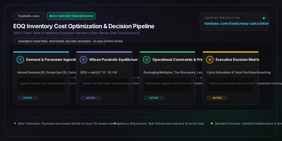
Kpi eoq419 Unit units
Kpi orders per year35.8 Lbl turns per year
Kpi cycle days10 Unit days
Kpi total relevant cost$3,224.13
Lbl reorder trigger point625 Unit units
Kpi parity ratio100.0%
Technical Reference & Architecture Guide

EOQ Calculator & Inventory Holding Cost Guide

Calculate economic order quantity (EOQ), optimal batch size, and annual holding costs. Minimize ordering expenses with reorder point and discount tier analysis.

EOQ Calculator & Inventory Holding Cost Guide — Client-Side In-Memory Architecture & Data Flow

Key Parameters & Controls

Annual Unit Demand (D)Annual Unit Consumption

Total non-negative unit demand forecasted over a standard 12-month fiscal period. Excludes obsolete stock write-offs and consignment inventory.

Default: 10,000 units/year
Fixed Order Setup Cost (S)Currency per Purchase Order

Marginal administrative cost per transaction: purchasing labor, purchase order generation, EDI transaction fees, inbound receiving dock inspection, and bill-of-lading processing. Excludes unit freight if freight is charged per piece.

Default: $50.00 / order
Unit Purchase Price (C)Monetary Wholesale Acquisition Cost

Net delivered cost per individual unit from the vendor before holding or internal overhead allocations. Must reflect net of supplier trade discounts.

Default: $25.00 / unit
Annual Carrying Charge Rate (i)Annualized Holding Percentage

Standard corporate hurdle rate spanning cost of working capital (WACC: 8%-14%), dedicated warehousing footprint (2%-5%), ad valorem taxes & insurance (1%-3%), and shrinkage/obsolescence reserves (3%-10%). Industrial financial benchmark ranges from 18% to 32%.

Default: 22% / year
Supplier Lead Time (L)Elapsed Transit Days

Verified elapsed calendar days between electronic purchase order release and validated warehouse dock put-away readiness.

Default: 14 days
Service Level Factor (Z)Statistical Standard Normal Deviate

Statistical coverage factor defining stockout tolerance during replenishment lead time: Z=1.282 for 90%, Z=1.645 for 95%, Z=1.960 for 97.5%, and Z=2.326 for 99.0% cycle service levels.

Default: 1.645 (95% Service Level)

Pro Tips & Best Practices

The Wilson 'Flat Bottom' Rule & Packaging Multiples

The Total Relevant Cost curve is remarkably flat near its parabolic minimum. Deviating by +/-15% from theoretical mathematical EOQ increases total annual inventory cost by less than 1.1%. Never order fractional pieces or break master carton packs—rounding EOQ to the nearest pallet or master case pack (e.g. 24 or 48 units) eliminates broken-carton warehouse fees with negligible holding impact.

Unbundling Cost of Capital vs Physical Storage Space

Do not treat holding cost as a single monolithic percentage if physical storage is constrained. Capital cost (WACC) scales strictly with inventory dollar value, whereas warehouse pallet storage scales with cubic physical volume. For bulky low-cost SKUs (e.g. insulation foam), physical cubic space dominates; for compact high-cost SKUs (e.g. microprocessors), capital interest rate dominates.

The Freight Cliff Effect vs True Order Cost

Traditional EOQ assumes order setup cost (S) is strictly fixed per order. In reality, freight carriers apply sharp rate cliffs between Less-Than-Truckload (LTL) and Full Truckload (FTL). If theoretical EOQ yields 18 pallets, rounding up to 24 pallets (1 full 53-ft dry van) often slashes freight cost per unit by 40%, far outweighing the modest additional inventory carrying cost.

Price Break Hurdle: Do Not Overbuy Without Calculating Breakeven

Vendors often dangle a 5% unit discount for doubling order quantities. To determine viability, calculate net profit delta: Annual Savings = [D * (C_old - C_new)] - [(Q_new * H_new / 2) - (EOQ * H_old / 2)]. If the additional holding cost on the trapped working capital exceeds annual purchase discount savings, rejecting the bulk discount preserves company liquidity.

Common Gotchas & Troubleshooting

⚠️Annual Holding Cost entered as a Percentage rather than a Dollar Value

Confirm your carrying cost input mode. If unit cost is $50 and carrying cost is 20%, the annual unit holding cost H is $10.00/unit/year. If entered erroneously as $0.20, calculated EOQ will inflate by over 700%, causing massive warehouse overstocking.

⚠️Calculated Order Frequency exceeds Operating Calendar Days

When annual demand is modest and setup cost is extremely low, mathematical EOQ can suggest ordering daily or multiple times per day. Constrain minimum cycle time to vendor minimum reorder intervals (e.g. weekly or bi-weekly batches).

⚠️Lead Time Demand exceeds Calculated EOQ

When supplier lead time is extended (e.g. 60-day overseas maritime transit), lead-time demand (d * L) often surpasses the cycle batch size (EOQ). In such pipeline inventory scenarios, Reorder Point (ROP) will be numerically greater than EOQ, requiring multiple open purchase orders concurrently in transit.

⚠️Warehouse Capacity Hard Ceiling Violation

Standard EOQ assumes infinite storage capacity. If peak inventory (EOQ + Safety Stock) exceeds allocated pallet racks, use the constrained EOQ solver: set maximum allowable batch size to (Max Rack Capacity - Safety Stock) and adjust replenishment frequency accordingly.

Frequently Asked Questions

How do you calculate Economic Order Quantity using the formula?▼

Economic Order Quantity is calculated using the classic Wilson formula: EOQ = sqrt((2 * D * S) / H), where D is annual unit demand, S is fixed order cost per purchase order, and H is annual holding cost per unit (H = Unit Cost * Carrying Rate %). For example, if annual demand is 10,000 units, order cost is $50, and holding cost is $5 per unit/year, EOQ = sqrt((2 * 10,000 * 50) / 5) = sqrt(200,000) = 447 units per order.

What is a normal holding cost percentage for inventory?▼

A standard annual inventory holding cost ranges between 20% and 30% of total inventory asset value per year. This rate comprises four financial components: Cost of Capital / WACC (8% to 15%), Storage & Facility Footprint (2% to 5%), Inventory Taxes & Insurance (1% to 3%), and Obsolescence, Shrinkage & Spoilage Reserves (3% to 8%). For perishable goods or fast-depreciating consumer electronics, carrying costs frequently exceed 35%.

What is the difference between EOQ and Reorder Point (ROP)?▼

EOQ determines 'how much' inventory to purchase in each batch to minimize combined ordering and carrying expenses, whereas Reorder Point (ROP) determines 'when' to trigger that purchase order based on supplier transit time. Reorder Point is calculated as: ROP = (Average Daily Demand * Lead Time Days) + Safety Stock. When on-hand plus on-order stock drops to the ROP threshold, an order of size EOQ is immediately placed.

Does EOQ still work when suppliers offer bulk quantity discounts?▼

Disclaimer: This tool is provided strictly for educational and informational purposes only and does not constitute formal financial advice or a binding loan commitment. Please consult a qualified financial advisor before making decisions. Standard EOQ must be adjusted when volume price breaks exist by evaluating Total Annual Cost at each price break tier: Total Cost = (D / Q) * S + (Q / 2) * H + (D * C). You first compute the standard EOQ at the discounted unit price; if that quantity qualifies for the discount, it is optimal. If not, evaluate total annual cost at the minimum quantity required for the discount (Q_discount) versus total cost at the baseline EOQ; choose whichever yields the lower total annual dollar expenditure.

Related Tools & Utilities

All Tools →