/

Nav title

Badge tier•Lbl cochran standard

Sample Size Calculator & Margin of Error

Calculate statistical sample size and margin of error for surveys or A/B tests with Cochran formula, finite population correction, and confidence interval curves.

Lbl quick pill bar

Title control deck

Lbl one prop model
Z = 1.96
±5.0%
±0.5% (Lbl high precision)±3.0% (Lbl gallup standard)±5.0% (Lbl standard precision)±10.0%
50%
10% (Lbl rare proportion)90% (Lbl prevalent proportion)
Txt infinite pop
1.0x
Lbl simple randomLbl moderate clusterLbl high cluster
20%

Hint drop off

Kpi required n
385

Kpi required n sub

95% Lbl confidence short
Kpi outreach
482

Kpi outreach sub

20% Lbl drop off short
Kpi std error
2.55%

Kpi std error sub

σ/√n
Kpi infinite pool
∞

Kpi infinite sub

Lbl cochran base

Title diminishing curve

Lbl sweet spot
n=385 (±5.0%)Lbl mo e y axisLbl sample size x axis

Desc diminishing

Title bell curve

Lbl confidence area: 95% (two-tailed)
-1.96α/2+1.96α/2
Title derivation
Lbl deriv step1n₀ = (Z² · p · (1-p) · DEff) / E²= (1.96² · 0.50 · 0.50 ) / 0.0500² = 385
Lbl deriv step2n = n₀ / [1 + (n₀ - 1) / N]Txt no correction needed
Lbl interval comparison
Lbl wald interval [45.0%, 55.0%]Lbl wilson interval [45.03%, 54.97%]
Stat cochran titleStat cochran desc
Stat privacy titleStat privacy desc
Stat export titleStat export desc

Client-Side Processing

High-performance calculation executed entirely in browser memory.

Zero Server Upload Privacy

All payloads remain strictly local with zero external server communication.

Production Ready Export

Clean, optimized output formats ready for immediate deployment.

Disclaimer title

Disclaimer text
Technical Reference & Architecture Guide

Sample Size Calculator & Margin of Error Guide

Calculate statistical sample size and margin of error for surveys or A/B tests with Cochran formula, finite population correction, and confidence interval curves.

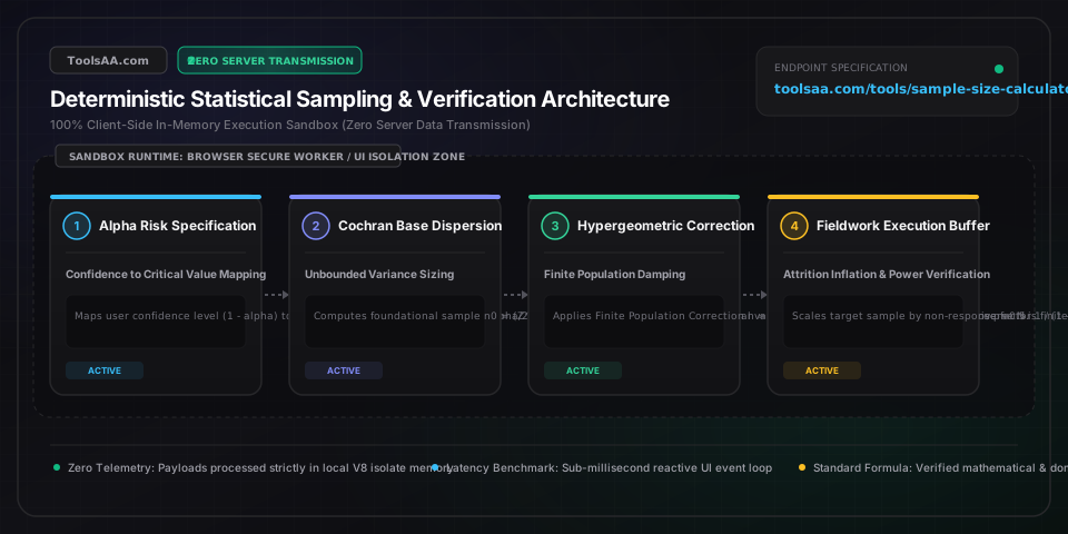
Sample Size Calculator & Margin of Error Guide — Client-Side In-Memory Architecture & Data Flow

Key Parameters & Controls

Confidence Level (1 - Alpha)Statistical Certainty Threshold

The long-run probability that repeated independent samples capture the true population parameter within the margin of error interval. Governed by the standard normal distribution critical value Z (90% = 1.645, 95% = 1.960, 99% = 2.576).

Default: 95%
Margin of Error (Absolute Radius E)Precision Bound Half-Width

The maximum acceptable expected difference between the observed sample statistic and the true population parameter. Halving the margin of error necessitates quadrupling the required sample size due to inverse-square mathematical mechanics.

Default: 5.0%
Population Proportion (Variance Prior p)Bernoulli Distribution Parameter

The assumed underlying proportion of the attribute under study. Setting p = 0.50 yields maximum mathematical variance p(1 - p) = 0.25, ensuring the most conservative upper-bound sample size recommendation.

Default: 50%
Population Universe Size (N)Finite Population Cardinality

Total number of entities in the study universe. When the sampling fraction (n / N) exceeds 5%, the Finite Population Correction (FPC) reduces required sample size without sacrificing statistical precision.

Default: Infinite
Statistical Power (1 - Beta)Hypothesis Detection Sensitivity

The probability of correctly rejecting the null hypothesis when a true alternative effect exists in A/B testing. Industry gold standard is set at 80% (Z_beta = 0.842) or 90% (Z_beta = 1.282) to avoid Type II false negative errors.

Default: 80%
Non-Response Attrition Rate (r)Fieldwork Execution Discount

The expected percentage of sampled participants who decline or fail to complete the survey instrument. Used to calculate total initial recruitment targets: n_invited = ceil(n / (1 - r)).

Default: 20%

Pro Tips & Best Practices

The Inverse-Square Quadrupling Law of Margin of Error

Precision does not scale linearly. Narrowing your margin of error from ±4% down to ±2% cuts the interval in half but requires multiplying your sample size by exactly four (from 601 to 2,401 respondents at 95% confidence). Budget field costs against this diminishing returns curve.

The 5% Finite Population Correction Threshold

If your total target universe N is large relative to your initial sample (specifically n0 / N < 0.05), applying the Finite Population Correction reduces the required sample size by less than 2.5%. You can safely use infinite population assumptions unless sampling dense, finite cohorts like corporate departments or niche medical patient pools.

The Conservative 50% Proportion Pitfall for Rare Events

Setting p = 0.50 is safe for political elections, but massively overestimates needed sample size when tracking rare occurrences (such as a 1% website checkout conversion or a 0.5% manufacturing defect rate). When measuring rare events, using a pilot estimate of p = 0.02 reduces required sample size by over 92%.

Non-Response Compounding Error vs Simple Multiplication

When accounting for a 40% non-response rate, do not add 40% to your sample size (n * 1.40). You must divide by the completion complement: n / (1 - 0.40) = n * 1.667. Multiplying by 1.40 leaves your field study 16% short of valid completions, compromising statistical power.

Common Gotchas & Troubleshooting

⚠️Required sample size exceeds total known population size

When precision requirements are set too strictly for small cohorts (e.g., ±1% error on N=300), Cochran base formulas yield n > N. The calculator automatically triggers Finite Population Hypergeometric bounds, capping the maximum sample size at N and recommending a 100% census.

⚠️Confidence interval endpoints fall outside the valid [0%, 100%] boundary

The standard Wald normal approximation interval p ± E degrades near extreme proportions (p < 0.05 or p > 0.95), generating impossible negative percentages. The tool automatically computes Wilson Score intervals with continuity correction to guarantee bounded intervals.

⚠️Central Limit Theorem violation warning for small samples

When n * p < 5 or n * (1 - p) < 5, sample distributions are heavily skewed and normal approximation critical values fail. The system alerts users to switch to Clopper-Pearson exact binomial calculations or increase sample size.

⚠️Traffic imbalance in A/B split testing degrades effective power

Deviating from an equal 50/50 split to a 90/10 traffic allocation drastically reduces effective statistical sample size. Sizing requirements increase by a factor of (1 + k)^2 / (4 * k) where k is the ratio of traffic allocations.

Frequently Asked Questions

How do you calculate sample size using Cochran's formula?▼

Cochran's sample size formula is n0 = (Z^2 * p * (1 - p)) / E^2, where Z represents the critical value from the standard normal distribution (1.96 for 95% confidence), p is the estimated proportion of an attribute in the population (0.5 for maximum variance), and E is the desired margin of error expressed as a decimal (0.05 for ±5%). For an infinite population with 95% confidence and 5% error, n0 = (1.96^2 * 0.5 * 0.5) / (0.05^2) = 384.16, rounded up to 385 respondents.

What is a good margin of error for a survey or poll?▼

A margin of error between ±3% and ±5% at a 95% confidence level is the standard benchmark for scientific public opinion polling, academic research, and commercial market surveys. High-stakes clinical, pharmaceutical, or regulatory testing typically requires tighter margins between ±1% and ±2%, whereas preliminary internal exploratory pulse checks often accept margins up to ±8% to minimize respondent acquisition costs.

What is the difference between confidence level and margin of error?▼

The confidence level measures how certain you are that your survey results reflect the population, expressed as the percentage of times repeated samples would encompass the true population value (typically 95%). The margin of error is the positive and negative numerical boundary around your sample percentage (such as ±3%). If a survey finds 60% customer approval with a ±3% margin of error at 95% confidence, it means that if the survey were repeated 100 times, 95 times the true approval would fall between 57% and 63%.

When should you use the finite population correction factor?▼

You should apply the Finite Population Correction (FPC) whenever your preliminary calculated sample size n0 constitutes more than 5% of your total target population N (n0 / N > 0.05). FPC calculates the adjusted sample size as n = n0 / (1 + (n0 - 1) / N). For example, if researching a company with 1,000 employees at a 95% confidence level and 5% margin of error, the base sample of 385 is reduced by FPC to 278, saving 107 interviews without losing accuracy.

How does non-response rate affect required sample size?▼

The required sample size calculated by statistical formulas represents completed, valid survey responses, not invitations sent. To achieve n completed surveys with an anticipated non-response rate r, the total recruitment outreach must be calculated as n_invited = ceil(n / (1 - r)). If your formula calls for 400 completed responses and your expected survey completion rate is 25% (a 75% non-response rate), you must distribute invitations to 400 / (1 - 0.75) = 1,600 prospective participants.

Related Tools & Utilities

All Tools →