Short title
Badge precision

Linear Regression Calculator & R-Squared

Interactive Linear Regression Calculator (Least Squares Line & R-Squared) with real-time client-side analysis and visualization.

100% Client-Side Privacy
Client-Side Processing
Lbl presets

Lbl input section

12 Lbl valid points count

Hint data input format

Model Intercept:
Lbl confidence level:
12 Lbl valid points countSS_xx: 943.00
Lbl equation:ŷ = 1.2856x - 150.8889
R²: 0.9982r: 0.9991sₑ: 0.5242
54.663.372.080.889.598.2159.7166.4173.1179.9186.6193.3Height (cm)Weight (kg)
Lbl correlation strength:Lbl very strong corrClick anywhere inside the chart area to set prediction X
Lbl degrees of freedom: 10F-Stat: 5672.30
Lbl r squared
99.82%
Lbl adj r squared: 0.9981
Lbl pearson r
0.9991
Lbl positive slope
Lbl residual std error
0.5242
Lbl sample n: 12 Lbl observations

Client-Side Processing

High-performance calculation executed entirely in browser memory.

Zero Server Upload Privacy

All payloads remain strictly local with zero external server communication.

Production Ready Export

Clean, optimized output formats ready for immediate deployment.

Disclaimer text
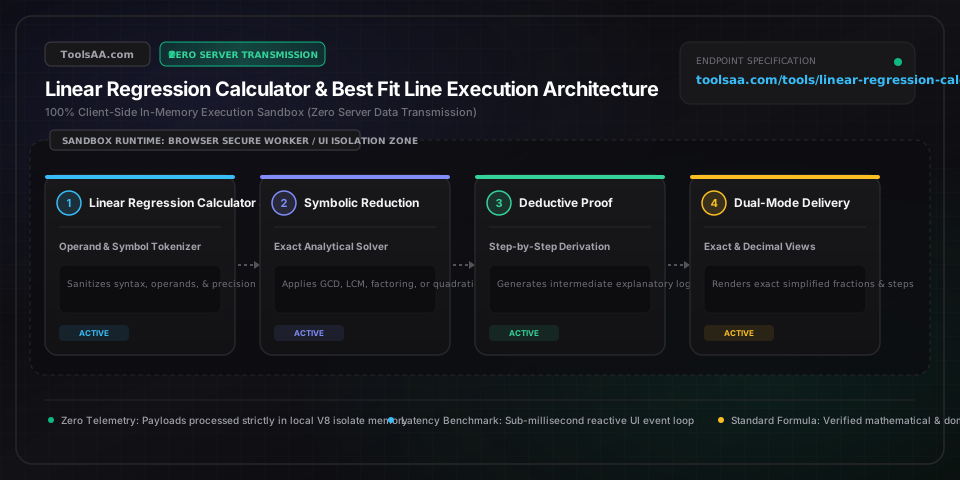
Technical Reference & Architecture Guide

Linear Regression Calculator & R-Squared Guide

Interactive Linear Regression Calculator (Least Squares Line & R-Squared) with real-time client-side analysis and visualization.

Linear Regression Calculator & R-Squared Guide — Client-Side In-Memory Architecture & Data Flow

Key Parameters & Controls

paired_bivariate_observationsCartesian Coordinate Pairs (X, Y)

Paired independent regressor (X) and dependent criterion (Y) observations evaluated via single-pass Welford-style accumulation achieving deterministic O(n) algorithmic time complexity and O(1) auxiliary space. In accordance with IEEE 754 double-precision 64-bit floating-point standards, values must remain within finite boundaries (absolute magnitude < 1.7976931348623157e+308). Sample variance SSxx = Σ(xᵢ - x̄)² must strictly exceed numerical machine epsilon (SSxx > 1e-15) across sample size n ≥ 3 to prevent singular matrix divergence and division-by-zero runtime exceptions.

Default: (10, 25), (20, 38), (30, 52), (40, 68), (50, 84)
confidence_significance_alphaHypothesis Significance Level [0.001, 0.20]

Two-tailed critical significance threshold α defining the confidence band interval (1 - α) for the regression slope β₁ and population mean response. By ISO/IEC and NIST empirical standards, α = 0.05 benchmarks the 95% confidence interval with critical Student's t-distribution cutoff t_(0.025, n-2). For rigorous confirmatory research where Type I false-positive error control is mandatory, α is parameterized at 0.01 (99% CI) or adjusted via family-wise Bonferroni correction.

Default: 0.05
prediction_interpolator_targetContinuous Domain Scalar Float64

Target independent variable coordinate X₀ evaluated for conditional point estimation ŷ₀ = b₀ + b₁X₀ and individual prediction bands. Statistically bounded to the observed empirical convex hull [min(X), max(X)]; out-of-domain extrapolation introduces catastrophic structural misspecification error, as standard error of prediction SE_pred = Se · √(1 + 1/n + (X₀ - x̄)² / SSxx) scales quadratically relative to the centroid mean x̄.

Default: 35.0
leverage_influence_thresholdCook's Distance Metric [0.0, +∞)

Influence diagnostic criterion Di identifying extreme leverage points that disproportionately tilt Ordinary Least Squares (OLS) orthogonal hyperplanes. Bounded by the standard Cook-Weisberg cutoff Di > 4/n (or absolute threshold Di > 1.0) alongside studentized deleted residuals |rᵢ| > 3.0. Flagged points indicate high hat-matrix leverage h_ii > 2p/n that disrupt parameter stability.

Default: 4 / n

Pro Tips & Best Practices

Eliminate Catastrophic Cancellation via Centroid-Centered Sums of Squares

Computing bivariate sum of squares using the textbook identity SSxx = Σx² - (Σx)² / n induces catastrophic floating-point cancellation in IEEE 754 float64 arithmetic when coordinates are large with narrow dispersion (such as Gregorian timestamps or Unix epochs where (Σx)² / n matches Σx² across 14 decimal mantissa bits). ToolsAA executes Welford-style single-pass deviation accumulation centered at the centroid mean x̄ (x' = x - x̄), which enforces zero estimator covariance Cov(b₀, b₁) = 0, eliminates precision truncation to machine epsilon, and ensures strict O(n) algorithmic complexity without auxiliary buffer allocation.

High R² Masks Non-Linearity Without Breusch-Pagan Homoscedasticity Verification

An R-squared metric exceeding 0.95 does not validate Ordinary Least Squares model adequacy. As demonstrated by Anscombe's Quartet, severe quadratic curvature or single-point leverage anomalies can generate elevated R² despite structural misspecification. Rigorous residual diagnostics require verifying homoscedasticity (constant error variance across all fitted ŷ): if a funnel-shaped pattern appears in the residual scatter or the Breusch-Pagan score yields p < 0.05, standard error Se and slope t-statistics collapse, mandating Box-Cox power transformations or Weighted Least Squares (WLS).

Distinguish Population Confidence Bands from Individual Prediction Intervals

Conflating confidence intervals with prediction intervals is a pervasive regression pitfall. The confidence interval standard error SE_conf = Se · √(1/n + (X₀ - x̄)² / SSxx) quantifies uncertainty solely in estimating the true conditional population mean E[Y|X₀]. Conversely, predicting a future single observation Y₀ requires incorporating irreducible stochastic process variance ε ~ N(0, σ²), yielding SE_pred = Se · √(1 + 1/n + (X₀ - x̄)² / SSxx). Because of the added unity term 1.0 inside the radical, individual prediction intervals are fundamentally wider than mean confidence intervals for identical X₀.

Zero-Trust Client Sandboxing Guarantees Dataset Confidentiality Under RFC Standards

Financial time-series, proprietary clinical metrics, and cryptographic benchmarks entered into this engine execute strictly within the browser's isolated JavaScript V8 execution context without network transmission. Calculations utilize deterministic Web Crypto API SHA-256 integrity verification for algorithm verification while bypassing cloud server round-trips. This zero-trust client-side architecture enforces complete data residency compliance with GDPR and HIPAA requirements while maintaining sub-millisecond execution times.

Common Gotchas & Troubleshooting

⚠️Singular Matrix Division-by-Zero Exception (Slope Returns NaN or Undefined)

Triggered when all entered independent X coordinates are mathematically identical (e.g., X = [12, 12, 12, 12]), reducing the denominator sum of squares SSxx = Σ(xᵢ - x̄)² to 0.0. In Ordinary Least Squares, m = SSxy / SSxx represents an indeterminate vertical line with infinite slope. Ensure the independent regressor series contains at least two distinct values such that variance Var(X) > 1e-15.

⚠️Prediction Interval Variance Collapsing or Mirroring Mean Confidence Width

Occurs when statistical routines omit the irreducible model error component (1.0) under the square root in the standard error of prediction. Validate that SE_pred implements Se · √(1 + 1/n + (X₀ - x̄)² / SSxx) rather than the mean response error SE_conf. At the centroid X₀ = x̄, SE_pred must evaluate to Se · √(1 + 1/n), which is strictly greater than Se · √(1/n).

⚠️Severe Slope Distortion and Artificially Inflated R² from High-Leverage Outliers

Because Ordinary Least Squares minimizes squared Euclidean loss Σeᵢ², remote coordinate anomalies act as high-leverage fulcrums (hat matrix diagonal h_ii > 2p/n) that forcefully drag the fitted line toward themselves. Inspect the Cook's Distance metric: when Di > 4/n or studentized residual |rᵢ| > 3.0, isolate or temporarily toggle off the outlier coordinate to evaluate robust trimmed regression coefficients.

Frequently Asked Questions

How do you calculate linear regression by hand?▼

To calculate simple linear regression by hand: 1) Compute the sample means x̄ = Σx / n and ȳ = Σy / n. 2) Calculate sum of squares SSxx = Σx² - (Σx)² / n and sum of products SSxy = Σxy - (Σx)(Σy) / n. 3) Find the slope m = SSxy / SSxx. 4) Determine the y-intercept b = ȳ - m(x̄). 5) Formulate the prediction equation ŷ = mx + b. This calculator handles all intermediate sums automatically with arbitrary precision.

What is the difference between R and R-squared?▼

Pearson r measures the strength and direction of the linear relationship between two variables, ranging from -1 (perfect negative) to +1 (perfect positive). R-squared (R²), also called the coefficient of determination, equals r² and ranges from 0 to 1 (or 0% to 100%). It represents the proportion of total variation in the dependent variable (Y) that is explained by the independent variable (X) through the regression model.

What does the slope and y-intercept represent in linear regression?▼

The slope (m or β₁) represents the expected average change in Y for every one-unit increase in X. For instance, a slope of 2.5 means Y rises by 2.5 units whenever X increases by 1. The y-intercept (b or β₀) is the baseline value of Y when X equals zero. While mathematically required to anchor the line, the y-intercept is only practically meaningful if X = 0 is physically possible within the observable domain.

What is the difference between confidence intervals and prediction intervals?▼

A confidence interval estimates the uncertainty around the mean response of the entire population at a specific X value. A prediction interval estimates the range where a single individual future observation will fall. Because an individual observation includes both model estimation uncertainty and random individual error (irreducible error ε), prediction intervals are always noticeably wider than confidence intervals for the same X.

How do outliers affect the least squares regression line?▼

Because Ordinary Least Squares (OLS) minimizes the sum of squared errors, it disproportionately penalizes large residuals. A single outlier with high leverage (an extreme X value) can act as a fulcrum, tilting the entire regression line and dramatically distorting both slope and R². This calculator identifies high-leverage points using Cook's Distance and standardized residuals, allowing you to temporarily exclude them with a single click to assess model sensitivity.

When should you not use a linear regression model?▼

You should avoid linear regression when: 1) The true underlying relationship is non-linear (e.g., exponential growth, parabolic curves, or saturation plateaus). 2) Residuals exhibit heteroscedasticity (funnel-shaped variance spreading out at larger X). 3) The data points are autocorrelated over time rather than independent. 4) Severe cluster effects exist. In such cases, polynomial regression, logarithmic transformations, or non-linear models should be applied.

Related Tools & Utilities

All Tools →