/
Probability Calculator & Odds Solver
Lbl mode singleTier M • L3 Dashboard

Probability Calculator & Odds Solver

Calculate single and multiple event probabilities, odds ratios, conditional Bayes outcomes, and independent or mutually exclusive event series with steps.

Lbl quick benchmarks:

Title control deck

50.00% (0.5000)
%:
Dec:
Lbl quick benchmarks
Lbl chance of event50.00%0.5000
Lbl complementary chance50.00%0.5000
Lbl odds in favor1:11/1 UK
Lbl natural frequency phrasing1 in 2Lbl trials suffix

Title decision cockpit

Lbl privacy badge
0% (Impossible)50.00%100% (Certain)
Decimal Multiplier2.00x
UK Fractional1/1
US Moneyline-100

Title step by step

Kolmogorov Axiom 1: Probability is strictly bounded between 0 and 1. P(A) = 0.5000.

Complementary Event: The chance of this not occurring is P(A') = 1 - P(A) = 0.5000 (50.00%).

Natural Frequency: In simple terms, this event occurs approximately once in every 2 attempts.

Lbl zero server latencyLbl client side math
Lbl complete health privacyLbl zero diagnostics uploaded
Lbl deterministic precisionLbl log gamma engine

Client-Side Processing

High-performance calculation executed entirely in browser memory.

Zero Server Upload Privacy

All payloads remain strictly local with zero external server communication.

Production Ready Export

Clean, optimized output formats ready for immediate deployment.

Disclaimer text

Technical Reference & Architecture Guide

Probability Calculator & Odds Solver Guide

Calculate single and multiple event probabilities, odds ratios, conditional Bayes outcomes, and independent or mutually exclusive event series with steps.

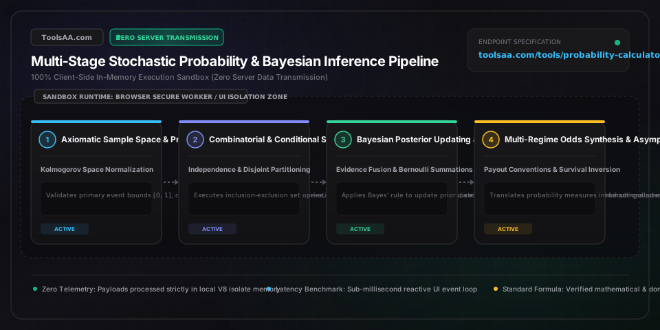
Probability Calculator & Odds Solver Guide — Client-Side In-Memory Architecture & Data Flow

Key Parameters & Controls

Event Probability P(A) & Axiomatic Sample SpaceDimensionless Real Ratio [0.000000, 1.000000]

The fundamental measure of likelihood that a specific event occurs within a defined sample space S. Governed by the Kolmogorov Axioms: non-negativity P(A) >= 0, unitarity P(S) = 1, and additivity for mutually exclusive events. Expressed identically as a decimal between 0 and 1, a percentage between 0% and 100%, or an irreducible integer ratio of favorable outcomes to total equally likely outcomes.

Default: 0.5000 (50.0%)
Joint Probability P(A and B) & Stochastic IndependenceJoint Set Measure [0.000000, 1.000000]

The probability of both event A and event B occurring simultaneously in a single trial or composite experiment. If events are independent, P(A intersect B) = P(A) * P(B). If dependent, P(A intersect B) = P(A) * P(B|A). The value is strictly bounded above by min(P(A), P(B)) and below by max(0, P(A) + P(B) - 1) according to Frechet inequalities.

Default: 0.0833 (8.33%)
Union Probability P(A or B) & Inclusion-ExclusionUnion Set Measure [0.000000, 1.000000]

The likelihood that at least one of the events occurs. Computed via the Principle of Inclusion-Exclusion: P(A union B) = P(A) + P(B) - P(A intersect B). When events are mutually exclusive (disjoint), the intersection term vanishes, simplifying to direct summation P(A) + P(B).

Default: 0.5833 (58.33%)
Conditional Probability P(A|B) & Bayesian LikelihoodNormalized Subspace Probability [0.000000, 1.000000]

The updated probability of event A occurring given that event B is known to have already occurred: P(A|B) = P(A intersect B) / P(B), where P(B) > 0. In Bayesian analysis, this represents the posterior probability after updating prior beliefs P(A) with the observed empirical likelihood P(B|A).

Default: 0.5000 (50.0%)
Odds in Favor (X:Y) & Odds AgainstCoprime Integer Ratio / Relative Likelihood

The ratio of the probability that an event occurs to the probability that it does not occur: Odds in Favor = P(A) / (1 - P(A)). A 75% probability corresponds to odds in favor of 3 to 1 (3:1). Odds against represent the reciprocal ratio (1 - P(A)) / P(A), universally employed in gaming and contract underwriting.

Default: 1:1 (Even Odds)
Bernoulli Trial Count (n) & Target Successes (k)Discrete Repetition Count (n >= 1, 0 <= k <= n)

Parameters governing binomial experiments consisting of n independent and identically distributed (i.i.d.) trials, each with constant binary success probability p. Combinatorial combinations C(n, k) determine the total permutations yielding exactly k successes.

Default: n = 10 trials, k = 5 successes
Bayes Base Rate Prior P(Hypothesis)Prevalence Baseline Proportion [0.000001, 1.000000]

The initial baseline probability of an event or medical condition before incorporating diagnostic test evidence. Ignoring this base rate leads to the Base Rate Fallacy, wherein high-accuracy tests yield paradoxically low positive predictive values when screening rare phenomena.

Default: 0.0010 (0.1% Prevalence)
Pro Tips & Best Practices

The Base Rate Fallacy in Medical Testing and Fraud Detection

When screening for a condition with a 0.1% population prevalence using a test that is 99% accurate (99% sensitivity and 99% specificity), a positive test result does not mean you have a 99% chance of having the disease. In a cohort of 100,000 individuals, 100 have the disease (99 test positive) while 99,900 do not (999 test false positive). The real posterior probability of actually having the condition given a positive test is only 99 / (99 + 999) = 9.01%.

The Gambler's Fallacy and Independent Bernoulli Trials

A streak of 10 consecutive coin tosses landing on Red or Heads does not increase the probability of Black or Tails on the 11th toss. Because physical fair coin flips possess zero memory (memorylessness), the conditional probability P(Heads_11 | 10 Heads) remains exactly 0.50. The Law of Large Numbers operates by dilution across future millions of trials, never by actively compensating or correcting for past short-term variances.

Bookmaker Overround and True Implied Probability Extraction

Commercial sportsbooks and betting exchanges artificially inflate betting odds so that the sum of implied probabilities across all outcomes exceeds 100% (typically 104% to 112%, known as the overround or vigorish). To calculate the true, fair statistical probability of an outcome, sum the individual implied probabilities (P_total = sum(1 / Decimal_Odds_i)) and normalize each runner: True Probability = (1 / Decimal_Odds) / P_total.

Common Gotchas & Troubleshooting

⚠️Sum of Union Probabilities Exceeding 1.00 (100%)

Adding P(A) and P(B) directly when events are not mutually exclusive double-counts their overlapping intersection P(A intersect B). If P(A) = 0.70 and P(B) = 0.60, the direct sum is 1.30, which violates Kolmogorov's first axiom. The correct probability of at least one event occurring is P(A union B) = 0.70 + 0.60 - P(A intersect B). Verify whether events can occur simultaneously before selecting the disjoint addition rule.

⚠️Assuming '95% Cumulative Probability' Guarantees an Event Occurs

In repeating a 1% chance event 298 times, the probability of at least one success is 1 - (0.99)^298 = 95.02%. However, this leaves an exact 4.98% residual probability of complete failure across all 298 attempts. Probability distributions are asymptotic and never reach 100% certainty with finite trials under continuous geometric survival functions. Plan sample sizes based on risk tolerance rather than expectations of an absolute guarantee.

⚠️Confusing Conditional P(A|B) with Inverse Conditional P(B|A)

This error (known as the Transposed Conditional or Prosecutor's Fallacy) confuses the probability of evidence given guilt with the probability of guilt given evidence. For example, P(Cloudy | Rain) is nearly 100%, but P(Rain | Cloudy) is only around 20% to 30%. Always use Bayes' theorem with the baseline prior rate to invert conditional statements: P(A|B) = [P(B|A) * P(A)] / P(B).

⚠️Extreme Sample Size Limits in Multi-Trial Binomial Series

Evaluating combinations C(n, k) for trials exceeding n = 170 causes arithmetic overflow in standard calculation engines because 171! exceeds mathematical magnitude limits (1.79e+308). For large trial experiments (such as n = 1,000 lottery draws or quality control batches), use logarithmic gamma transformations: ln C(n, k) = lnGamma(n + 1) - lnGamma(k + 1) - lnGamma(n - k + 1), which preserves precision across any trial volume without calculation failure.

Frequently Asked Questions

How do you calculate the probability of two independent events both occurring?▼

To calculate the probability of two independent events both occurring, multiply their individual probabilities together: P(A and B) = P(A) * P(B). For example, the probability of flipping Heads on a fair coin (0.50) and rolling a 6 on a fair six-sided die (1/6 = 0.1667) is 0.50 * 0.1667 = 0.0833, or exactly 8.33% (1 in 12).

What is the difference between odds and probability?▼

Probability measures the ratio of favorable outcomes to all possible outcomes, bounded between 0 and 1 (or 0% to 100%), while odds represent the ratio of favorable outcomes to unfavorable outcomes. For example, rolling a 4 or higher on a standard six-sided die has a probability of 3/6 = 50% (0.50), but the odds in favor are 3 to 3, simplified to 1:1 even odds. To convert any probability P into odds in favor, divide P by (1 - P).

How many attempts are needed to guarantee a 99% chance of success?▼

To reach a 99% cumulative probability for an event with single-trial success chance p, calculate attempts using n = ceil(ln(1 - 0.99) / ln(1 - p)). For a 1% success rate (p = 0.01), this requires n = ceil(ln(0.01) / ln(0.99)) = 459 consecutive attempts. While 459 trials yield a 99.01% likelihood of at least one success, finite trials can never reach an absolute 100% mathematical guarantee due to asymptotic failure probability.

How does Bayes' theorem update probability with new evidence?▼

Bayes' theorem updates an initial prior probability using the formula P(A|B) = [P(B|A) * P(A)] / P(B), where P(A) is your baseline prior belief, P(B|A) is the likelihood of observing the evidence given the condition, and P(B) is the total probability of the evidence occurring across all scenarios. This mathematically transforms prior odds into updated posterior odds by multiplying the prior belief by the Bayes Factor (likelihood ratio).

Why does the Gambler's Fallacy cause people to miscalculate odds?▼

The Gambler's Fallacy is the mistaken belief that past independent events influence future outcomes in a random process. If a roulette wheel lands on black 8 times in a row, the probability of black on the 9th spin remains identical (18/38 or 47.37% on an American wheel). Independent random events have no memory, meaning past streaks create no mathematical imbalance that nature must correct in subsequent trials.

How do you convert American moneyline odds to implied probability?▼

For negative American odds (betting favorites, e.g., -200), implied probability equals |Odds| / (|Odds| + 100), yielding 200 / (200 + 100) = 66.67%. For positive American odds (underdogs, e.g., +250), implied probability equals 100 / (Odds + 100), yielding 100 / (250 + 100) = 28.57%. To calculate the true fair probability without the house edge (vigorish), divide the outcome's implied probability by the sum of all market probabilities.

Related Tools & Utilities

All Tools →